How to use vcdisk
This page demonstrates how to use vcdisk in typical use cases in Astronomy.
What is vcdisk?
vcdisk uses the method of Casertano (1983) to solve Poisson’s equation on the mid-plane of a thick axisymmetric galaxy disk. This is a fast and efficient way to compute the circular velocity of a stellar/gas disk with an arbitrary surface density distribution.
Why do we need vcdisk?
The most typical use case for vcdisk is in rotation curve modelling. Specifically, this module allows to compute the contribution to the circular velocity of the observed baryonic components of a disk galaxy, e.g. the stellar disk, the gas disk, the stellar bulge.
If we have some kinematical observations that allowed us to measure the rotational velocities of some material in circular orbits in the disk of a spiral galaxy (e.g. cold gas), the observed rotation curve can be decomposed into several dynamically important components in the galaxy 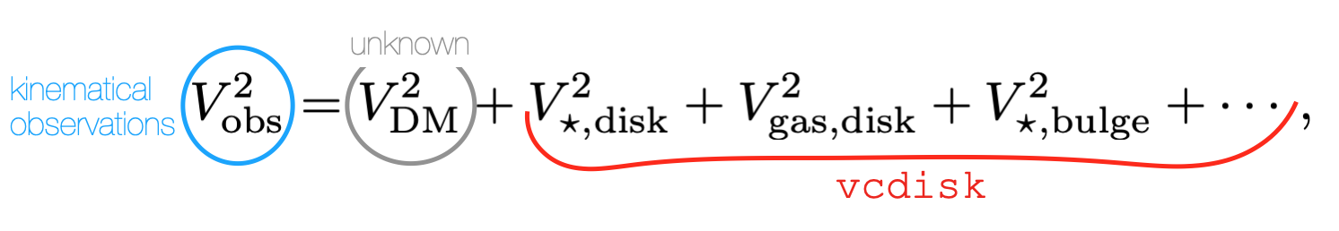 where \(V_{\rm DM}\) is the contribution from dark matter, \(V_{\star,\rm disk}\) from the stellar disk, \(V_{\rm gas, disk}\) from the gas disk etc. While the left-hand
side of this equation usually comes from observations, and the contribution of DM is the unknown that is often what we want to constrain, for all the other terms there is
where \(V_{\rm DM}\) is the contribution from dark matter, \(V_{\star,\rm disk}\) from the stellar disk, \(V_{\rm gas, disk}\) from the gas disk etc. While the left-hand
side of this equation usually comes from observations, and the contribution of DM is the unknown that is often what we want to constrain, for all the other terms there is vcdisk!
vcdisk calculates the contribution to the gravitational field of an axisymmetric component whose radial surface density distribution is known. For instance, the surface density profiles of stellar (\(\Sigma_{\star, \rm disk}\)) and gaseous disks (\(\Sigma_{\star, \rm disk}\)) can be directly obtained from galaxy images in appropriate wavebands and these can then be used as input for vcdisk to calculate \(V_{\rm disk}(R, \Sigma_{\rm disk}(R))\).
While the method of Casertano (1983) is designed for thick disks it works for all flattened axisymmetric distribution. Hence, it is ideal also to derive the contribution to the circular velocity of a flattened (pseudo-)bulge.
Example 1: analytic surface density
Import vcdisk
[1]:
from vcdisk import vcdisk

import numpy as np
import matplotlib.pylab as plt
Exponential thick disk
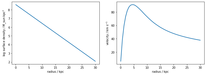
Let’s start with the case of a thick disk with a classical exponential surface density.
[2]:
md, rd = 1e10, 2.0                        # mass, scalelength of the disk
r = np.linspace(0.1, 30.0, 50)            # radii samples

def expdisk_sb(r, md, rd):
    # exponential disk surface density
    return md / (2*np.pi*rd**2) * np.exp(-r/rd)

sb_exp = expdisk_sb(r, md, rd)

# run vcdisk
vdisk = vcdisk(r, sb_exp)
[3]:
def plot_sb_vdisk(ax, r, sb, vdisk, label=None):
    ax[0].plot(r, np.log10(sb), lw=2)
    ax[0].set_xlabel("radius / kpc");
    ax[0].set_ylabel("log surface density / M_sun kpc"+"$^{2}$");

    ax[1].plot(r, vdisk, lw=2,  label=label)
    ax[1].set_xlabel("radius / kpc");
    ax[1].set_ylabel("velocity / km s"+"$^{-1}$");
    if label is not None: ax[1].legend()

fig,ax = plt.subplots(figsize=(12,4), ncols=2)
plot_sb_vdisk(ax, r, sb_exp, vdisk)
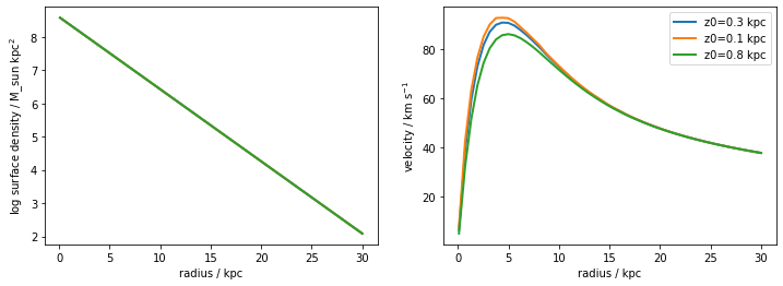
We can explore how does \(V_{\rm disk}\) change when changing the scaleheight of the disk \(z_0\) for instance:
[4]:
fig,ax = plt.subplots(figsize=(12,4), ncols=2)
plot_sb_vdisk(ax, r, sb_exp, vdisk, label='z0=0.3 kpc')
plot_sb_vdisk(ax, r, sb_exp, vcdisk(r, sb_exp, z0=0.1), label='z0=0.1 kpc')
plot_sb_vdisk(ax, r, sb_exp, vcdisk(r, sb_exp, z0=0.8), label='z0=0.8 kpc')
Sersic profile
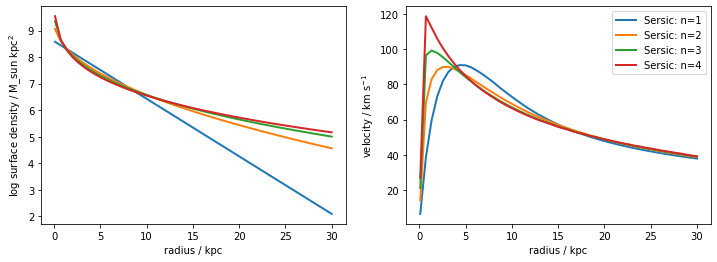
Let’s compare to other popular analytic surface density profiles. Probably the most used in Astronomy is the Sersic (1968) profile, which is often used to describe all sorts of stellar components, including disks and bulges.
[5]:
def sersic(r, Ie, Re, n):
    bn = 2*n -1./3. +4./405./n # Ciotti & Bertin (1999): https://ui.adsabs.harvard.edu/abs/1999A%26A...352..447C/
    return Ie * np.exp(-bn * ((r/Re)**(1/n)-1))
Let’s take as a reference the model:
[6]:
sb_sers_disk = sersic(r, 0.743e8, 1.678*rd, 1.0)
which is equivalent to the exponential disk that we have above. Let’s now compare the circular velocities of disks with Sersic surface brightnesses with different index \(n\), while keeping the total luminosity fixed.
[7]:
# here the profiles are renormalized to yield the same total mass = 1e10 Msun
# see e.g. Eq.(2) in Graham & Driver (2005): https://ui.adsabs.harvard.edu/abs/2005PASA...22..118G
sb_sers_n4 = sersic(r, 0.392e8, 1.678*rd, 4.0)
sb_sers_n3 = sersic(r, 0.449e8, 1.678*rd, 3.0)
sb_sers_n2 = sersic(r, 0.545e8, 1.678*rd, 2.0)

fig,ax = plt.subplots(figsize=(12,4), ncols=2)
plot_sb_vdisk(ax, r, sb_sers_disk, vcdisk(r, sb_sers_disk), label='Sersic: n=1')
plot_sb_vdisk(ax, r, sb_sers_n2, vcdisk(r, sb_sers_n2), label='Sersic: n=2')
plot_sb_vdisk(ax, r, sb_sers_n3, vcdisk(r, sb_sers_n3), label='Sersic: n=3')
plot_sb_vdisk(ax, r, sb_sers_n4, vcdisk(r, sb_sers_n4), label='Sersic: n=4')
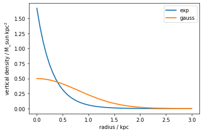
User-defined vertical density profile
vcdisk allows us to specify our own vertical density profile, if we so choose. This can be easily done through the rhoz argument.
[8]:
def rhoz_gauss(z, m, std): return np.exp(-0.5*(z-m)**2/std**2) / np.sqrt(2*np.pi*std**2)

def plot_rhoz(ax, z, rhoz, label=None):
    ax.plot(z, rhoz, lw=2, label=label)
    ax.legend()
    ax.set_xlabel("radius / kpc");
    ax.set_ylabel("vertical density / M_sun kpc"+"$^{2}$");


fig, ax = plt.subplots(figsize=(6,4))
z = np.linspace(0,3)
plot_rhoz(ax, z, np.exp(-z/0.3) / (2*0.3), label='exp')
plot_rhoz(ax, z, rhoz_gauss(z, 0., 0.8), label='gauss')
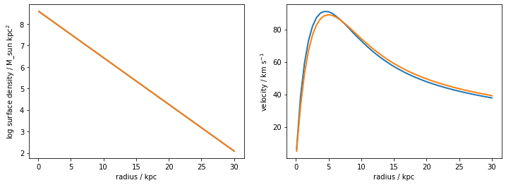
[9]:
fig,ax = plt.subplots(figsize=(12,4), ncols=2)

plot_sb_vdisk(ax, r, sb_exp, vdisk)
plot_sb_vdisk(ax, r, sb_exp, vcdisk(r, sb_exp, rhoz=rhoz_gauss, rhoz_args={'m':0.0, 'std':0.8}))
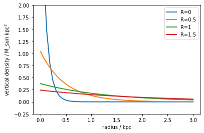
Flaring disk
We can also have a flaring disk, i.e. one where the vertical density depends also on radius \(\rho_z=\rho_z(z,R)\). We can work out this case as well with vcdisk by specifying how \(\rho_z\) depends on \(R\).
[10]:
def rhoz_exp_flaring(z, R, z00, Rs):
    z0R = z00+np.arcsinh(R**2/Rs**2)
    return np.exp(-z/z0R) / (2*z0R)

fig, ax = plt.subplots(figsize=(6,4))
z = np.linspace(0,3)
plot_rhoz(ax, z, rhoz_exp_flaring(z, 0.0, 0.1, 0.8), label='R=0')
plot_rhoz(ax, z, rhoz_exp_flaring(z, 0.5, 0.1, 0.8), label='R=0.5')
plot_rhoz(ax, z, rhoz_exp_flaring(z, 1.0, 0.1, 0.8), label='R=1')
plot_rhoz(ax, z, rhoz_exp_flaring(z, 1.5, 0.1, 0.8), label='R=1.5')
plt.ylim(None,2);
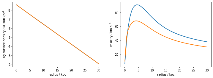
[11]:
fig,ax = plt.subplots(figsize=(12,4), ncols=2)

plot_sb_vdisk(ax, r, sb_exp, vdisk)
plot_sb_vdisk(ax, r, sb_exp, vcdisk(r, sb_exp, rhoz=rhoz_exp_flaring, rhoz_args={'z00':0.1, 'Rs':0.8}, flaring=True))
Example 2: observed surface brightness
Let’s say that, instead of having just simple galaxy images from which we can derive an analytic approximation for the galaxy surface brightness, we have a detailed galaxy image from which we can measure the intensity in elliptical annuli. This is for instance the case of nearby galaxies such as NGC 2403, that I use here as an example.
I use data taken from the SPARC database for this galaxy, which I include in this package as the NGC2403_rotmod.dat file. Here are reported measurements of the intensity at 3.6\(\mu\)m taken with the SPITZER space telescope in elliptical annuli for this target.
[12]:
rad, _, _, _, _, _, sb_n2403, _ = np.genfromtxt('NGC2403_rotmod.dat', unpack=True)
# convert SB to Msun / kpc^2
sb_n2403 *= 1e6
Now we can very easily use vcdisk to calculate \(V_{\star, \rm disk}\) for this galaxy, and we can evena compare it to some analytic profiles.
[13]:
vd_n2403 = vcdisk(rad, sb_n2403, z0=0.4)       # z0=0.4 kpc from Fraternali et al. (2002): https://ui.adsabs.harvard.edu/abs/2002AJ....123.3124F
sb_exp_n2403 = expdisk_sb(rad, 1.004e10, 1.39) # numbers taken from http://astroweb.cwru.edu/SPARC/

fig,ax = plt.subplots(figsize=(12,4), ncols=2)

plot_sb_vdisk(ax, rad, sb_exp_n2403, vcdisk(rad, sb_exp_n2403), label='exp-disk')
plot_sb_vdisk(ax, rad, sb_n2403, vd_n2403, label='observed')
/Users/lposti/anaconda/envs/py37/lib/python3.7/site-packages/ipykernel_launcher.py:2: RuntimeWarning: divide by zero encountered in log10
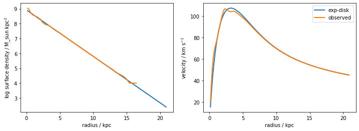
The \(V_{\star, \rm disk}\) curve obtained with vcdisk directly from the ellipse photometry of NGC 2403 is much more structured between \(1-5\rm \,kpc\), which is where the surface brightness has dips and peaks. Capturing this rich structure is essential to rotation curve modelling.
[ ]: